Interpolating data points to produce colour maps – code examples

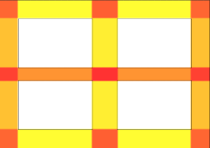
For a lot of the work I do in my research, I need to produce colour maps which can visualise data in a user-friendly way while still getting across the necessary elements of the analysis performed. In my current area of research, looking at wayfinding tools to analyse healthcare building design for natural wayfinding, I’m analysing and assigning values to nodes in early prototype development which highlight areas of a design which may be poor for natural wayfinding. However, visualising this by assigning one value to an entire area of the design produces a ‘blocky’ output which does not favourably portray the analysis results. As seen in the first image below, producing a colour map for sections based on one value produces colour maps which do not visualise the data very well.

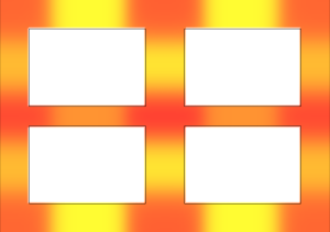
Difference between non-interpolated and interpolated colour map production

‘Blocky’ representation of the space

As seen in this image, the colour map is suggesting that people who step from one area to the next are going to have a drastically different experience in the space. But this isn’t the case, as some of the experience would ‘bleed over’ into the other areas. However, to compute a value for every point in the colour map would take such a long time that you might as well leave your analysis running overnight and hope for the result in the morning. This isn’t an ideal solution, so instead we can make use of interpolation algorithms to obtain data values for the mesh points from the control values that have been calculated. This is the basis for this post, to provide the code I have used to do this as I’ve used it many times in the past but always end up having to research how to use it as I usually forget. Hopefully this post will save me that research time and maybe save someone else as well.

When we use interpolation to produce the colour map, we end up with a visualisation like this:

Smooth representation of the space

This produces a colour map which favourable visualises the data, and suggests that changes are more gradual through the space. Overall, a better output for our data.

Interpolation Code

As the interpolation algorithm used at the moment is specific to my current research, I am giving the pseudo-code solution for interpolating data points so that when this is next needed (by myself or someone else) they won’t get bogged down in translating the specifics that I used (which is what pseudo-code should be used for of course).

For the interpolation to work, you need to work out the value based on the distance between the point you’re looking at ($latex C_{3}$) and the control points ($latex C_{1}$and $latex C_{2}$in this example). This is done by taking the weighted distance between $latex C_{1}$ and $latex C_{3}$, multiplying this by the value associated with $latex C_{1}$ and then repeating replacing $latex C_{1}$ with $latex C_{2}$. This is then divided by the sum of the weighted distances to produce the interpolated value for $latex C_{3}$.

$latex \&s=2 C_{3} = \frac{(C_{1} * \phi_{1}) + (C_{2} * \phi_{2})}{\phi_{1} + \phi_{2}}$

Where i refers to the weighted value (calculated below). Of course, if we have more than 2 control points, we can expand this very easily by just continually adding $latex C_{n}$ and $latex \phi_{n}$ to the formula.

$latex \&s=2 C_{u} = \frac{\sum_{i=1}^{n} C_{i}\phi_{i}}{\sum_{i=1}^{n}\phi_{i}}$

Weighting formula to calculate i

$latex \&s=2 \phi(r) = e^{-(\varepsilon r)^{2}} $

The distance between your control point and the point you’re looking at is multiplied by a weighting of your choice ($latex \varepsilon$) to become $latex \varepsilon r$. This is then squared and multiplied by the mathematical constant e.

For the purpose of the following pseudo-code, the mathematical constant e has been appropriated as 2.71828 – you can opt to find a definition for e in your chosen language or use more decimal places depending on the project you’re working on where you need this.

Pseudo-code

double WeightingFunction(double distance) {
    double r = pow( (0.35 * distance), 2 );
    return pow(2.71828, (-1 * r) );
}

This pseudo-code function takes the distance between the point being looked at and the current data point being looked at and returns the value associated for that data point.

Hopefully this helps someone produce smooth colour maps to visualise data, or at least helps me the next time I need to perform this operation. Thanks goes to James for his assistance in producing the weighting function required for the work I was doing at the time.